Scientific Computing Using Python - PHYS:4905
Lecture #22 - Prof. Kaaret
Homework #16 is at the bottom of this page.
Squaring the circle
Numerical integration is the use of an algorithm to calculate the
value of a definite integral. It is also refereed to as quadrature,
which is a historical mathematical term that means calculating area
of a geometric shape by constructing a square with the same
area. The "quad" is the same root that leads us to use the
name quadratic for a polynomial in which the highest power
is a square. People have been working on quadrature since
Babylonian times. There is a papyrus from Egypt from around
1550 BC that states that "a circle's area stands to that of its
circumscribing square in the ratio 64/81". If you think
about this, it means that the Egyptians knew the value of π to an
accuracy of 0.6%.
Trapezium
We will consider the problem of finding an approximate numerical
value of the integral of a function f(x), the
integrand, over an interval [a, b],
We evaluate the function at n+1 points equally distributed
in [a, b]. The spacing between adjacent points
is then Δx = (b-a)/n. and the x-values
are xk = a +k Δx, where k
= 0, 1, ..., n.
A simple algorithm would be approximate each interval by a rectangle
with a width of Δx and a height equal to value of the
function at the left edge. This is called a left Riemann
sum. As you can see from the figure below. The left
Riemann sum is not a great way to calculate an integral. It
works if you make your bins fine enough (at the cost of more
computations), but it underestimates the integral in regions where
the function slope is positive and overestimates it where the slope
is negative. One could instead use a right Riemann sum, taking
the function value at the right edge, but it has the same issues,
only reversed.
A better thing to do is to use a trapeze. Oops, that's for the
circus. I meant a trapezium. The Trapezium is a tight
open cluster of stars in the heart of the Orion Nebula, named for
its four brightest stars.

Trapezium is also the word used in English outside North America to
denote a convex quadrilateral with at least one pair of parallel
sides. Most of us in this class call such an object a
trapezoid.
Trapezoids offer a more accurate way to estimate an integral.
The idea is that rather than draw a rectangle with a height set by
the function value at one edge, let's draw a trapezoid between the
two edges. For reasonably smooth functions, this often
provides a nice approximation to the function, and therefore a more
accurate estimate of its integral.
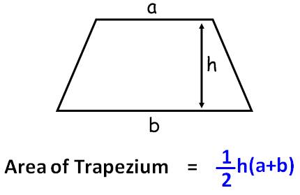
The area of a trapezoid is (a+b)h/2, where h is its height and a and
b are the lengths of the two sides.
We'll flip the trapezoid on its side, so that
.
The area of each trapezoid is then .
To calculate the integral, we sum the areas of all of the
trapezoids. For the first trapezoid, we'll have
When we add in the second one we get
Adding the third,
Note that we have to pay special attention to the first and last
points because they only contribute to one trapezoid while all of
the other points contribute to two.
Our approximation for the integral is then
Doing numerical integration this way is called using the trapezoid
rule and this formula is called the extended trapezoid rule.
We can write a Python function to do numerical integration via the
trapezoid rule using the following steps.
- Take as input, the name of the function to be integrated (f),
the endpoints of the interval of integration (a, b),
and the number of points to use (n).
- Create an array with xk values evenly
spaced from a to b.
- Evaluate the function at each xk value.
- Evaluate the sum in the equation above.
- Return the sum multiplied by the spacing between the points as
an estimate of the integral.
Thomas Simpson's rule
Approximating our function with trapezoids is nice, but it misses
sometimes, particularly if there is a maximum or minimum between our
x-values or the function has curvature. The trapezoid
rule approximates the integrand by drawing a line between adjacent
pairs of points. Instead, we could take adjacent triples of
points, draw a parabola through those three points, and integrate
that parabola analytically. This often does a better job as
nicely shown the figure below (drawn by Popletibus),
The formula for the area for one interval is
Note that if you substitute x0 = donut, x2
= beer, f(x)= Homer(x), you can re-write this
as Homer Simpson's rule,
To calculate the integral, we sum the integrals of all our little
parabolas. Note that we move by 2Δx each time so that
successive integration intervals don't overlap. The extended
Simpson's rule for calculating an integral is
The coefficients alternate between 4 and 2 all the way through the
middle of the sum. Note that n needs to be an even
number so that we have an odd number of terms in the sum.
The algorithm for doing integration via Simpson's rule is very
similar to that for the trapezoidal rule, but the sum is different.
Higher power?
You might ask, why stop at quadratic polynomials? There is a
Simpson's rule that uses cubic polynomials and the so-called
Newton–Cotes formulae allow any degree of polynomial. However,
one reaches diminishing returns because high order polynomials tend
to oscillate around the points they are drawn through and don't
actually provide better approximations. This is especially
true if the function has jumps, as seen in the figure below that
shows approximations to a step function with polynomials of 3rd,
5th, and 7th order and with the trapezoid rule. The trapezoid
rule clearly does a better job.
In general, numerical integration methods tend to work well for
smooth functions and poorly for functions with sharp features or
oscillations over scales close to the integration step size (Δx
in our discussions above). If your function has one or a few
discrete steps at known locations, then it is better to break the
integration up into pieces with edges at the step locations.
If your function oscillates, then you need to have at least
several integration bins within each oscillation period.
Adapt or perish
The accuracy of our estimation of the integral using either the
trapezoid rule or Simpson's rule is essentially set by the number of
grid points. More points means a smaller step size leading to
a better approximation of the function. The method don't
include a means to estimate the accuracy of the integration because
that depends on how well they approximate the function, which is
impossible to know precisely unless one can evaluate the integral
analytically, in which case one should do that rather than doing a
whole bunch of computations, or one evaluates the function at all
points in the integration interval, which would take an infinite
amount of time.
Usually, one estimates the accuracy by comparing the numerical
estimates obtained with different grid spacing. E.g. find the
integral using 1000 grid points, do it again with 2000 grid points,
and then take the absolute value of the difference as an estimate of
the accuracy. If the integrand is relatively smooth, so higher
order derivatives are not too large, then the accuracy of the
trapezoid rule scales with while
the accuracy of Simpson's rule scales with
.
You will check this in the homework assignment below.
In adaptive quadrature, the algorithm adjusts the grid to
obtain the desired accuracy. In simplest adaptive quadrature
algorithm, one
- Chooses an grid size and applies a method like the trapezoid
rule or Simpson's rule to estimate the integral. We'll
call the value of the integral I0.
- Divides the step size in half and repeats the numerical
integration. We'll call the new value of the integral I1.
- Checks if the desired accuracy has been reaches, specifically
check if abs(I1 - I0) <
itol*abs(I1), where itol is the
desired fractional accuracy. If we have reached the
desired accuracy, then we are done and we return I1.
If not, we set I0 = I1
and go back to step 2.
Such algorithms are called "globally" adaptive because they adjust
the whole grid. The trapezoidal rule and Simpson's rule are
particularly useful because we get to re-use all of the function
evaluations as we make the grid finer by dividing the step size in
half. The trapezoidal rule is particularly computationally
efficient because we don't even have to redo the sum over those
points.
becomes
We can simply add the old sum to the new sum with the new
points. We don't even have to keep the values from the
function evaluations on the coarser grid.
The disadvantage of globally adaptive quadrature is that the finer
grid spacings can become computationally expensive. In locally
adaptive quadrature, one breaks the interval into pieces and refines
the grid only for the pieces where the integral is not sufficiently
accurate. For example, one might
- Evaluate the integral in the intervals [a, (a+b)/2]
and [(a+b)/2, b], i.e. divide the original
interval in half, using a step size of Δx.
- Evaluate the integral in the same intervals using a step size
of Δx/2.
- For each of those intervals, check if we have reached the
desired accuracy using the same equation as in step 3 for global
quadrature. Note that if we achieve the desired fractional
accuracy in all intervals, then we will achieve it globally.
- For any interval where we have reached the desired accuracy,
stop and record the integral for that interval. For any
interval where we have not reached the desired accuracy, split
that interval into two pieces by going back to step 1 with a
and b set to the edges of that interval.
Some locally adaptive quadrature algorithms have an additional check
and stop if the global accuracy of the integral is good enough, i.e.
they add up the contributions from all of the pieces at each step
and stop if estimate of the total integral changes by less than itol
even if that accuracy hasn't been achieved for each individual
piece. This keeps the algorithm from throwing computational
resources into small pieces of the interval that are poorly behaved,
but don't make a large contribution to the total integral.
Locally adaptive quadrature is rather more complex to program than
globally adaptive quadrature. Most people don't even try, but
instead use a software package called QUADPACK that
was written in Fortran in the 1980s. There is a 300 page book
describing QUADPACK. Fortunately, the SciPy library includes
an interface to QUADPACK. The routine scipy.integrate.quad
uses locally adaptive quadrature to numerically integrate a
function, f(x), in a given interval (a, b),
to a specified relative accuracy epsrel, which is set by
default to 1.49e-08. It returns the value of the integral and
an estimate of the error. An example calling sequence is
from scipy.integrate import quad
integral, integral_err = quad(f, a, b)
The routine has many optional parameters and many more variables
that it can return that are described at its reference page https://docs.scipy.org/doc/scipy/reference/generated/scipy.integrate.quad.html.
There is also a version to do double integrals of functions with two
variables, scipy.integrate.dblquad.
Homework #16
For HW #15, you will write Python code to perform numerical
integration via the trapezoid rule and Simpson's rule and evaluate
the accuracy of those routines. Please hand in your code
electronically.
Your code should have a function integrate_trapezoid that
does numerical integration using the trapezoid rule and takes as
input: the name of the function to be integrated (f), the
endpoints of the interval of integration (a, b), and
the number of points to use (n). Write this function
first and test it by integrating
over the interval [0, 10], which you should be able to check
analytically. Your code should have a similar function integrate_simpson
that does numerical integration using Simpson's rule.
In the main body of your script, define the function
g(x) = (1+cos(x)) * exp(-x/(2*pi))
First plot this function over the interval x = [0, 60].
Then write a loop that integrates this function in the interval [0,
60] using different values for the number of points,
where j = 6, ... 16. Do the integration using both the
trapezoid rule and Simpson's rule.
For each n, plot the error in the numerical integration,
which we will define as the absolute value of the difference between
numerically calculated integral and the analytically calculated
integral which is
versus the integration step size, Δx. You should do
this on a log-log scale. Think about what trends you
see. In particular, does the error for each method depend on
some power of Δx? Include a comment block at the end
of your code with some discussion of this.
This assignment is worth 50 points.