Scientific Computing Using Python - PHYS:4905 - Fall 2018
Lecture #12 - 10/2/2018 - Prof. Kaaret
Image display and processing
Today we'll looking at processing and displaying images in
Python. Most of the code we'll examine involves calling
routines in various Python libraries. As discussed in lecture
#4, a large part of the effort in using libraries to perform tasks
is figuring out what function calls you need to make to do what you
want. The code that you'll use today are useful examples for
plotting images and histograms, making contour and surface plots,
and smoothing images.
M57 - the Ring nebula
The image we will use today was taken using the Hubble Space
Telescope and is of the object known as Messier 57 (M 57) and also
known as the Ring nebula. Objects like M57 are called
"planetary nebula" because they have a disk-like shape and look like
planets if viewed through a telescope with low resolution.
"Planetary" nebula have nothing to do with planets. The name
persists because astronomers are too steeped in their own history.

"Planetary" nebula are actually shells of gas expelled when a star
sheds it outer layers as it ends the giant phase of its evolution
and becomes a white dwarf - a hot, compact stellar remnant.
The white dwarf in the Ring nebula has a temperature of 1.2×10⁵
K and is visible as the white dot in the center. Ultraviolet
light from the white dwarf illuminates the surrounding gas.
The colors in the image are approximately true colors. The color
image was assembled from three images taken through different narrow
band filters with the Hubble telescope's Wide Field Planetary Camera
2. Blue isolates emission from very hot helium (filter is centered
at 469 nm to capture He II), which is located primarily close to the
hot central star. Green represents ionized oxygen ([O III] at 502
nm), which is located farther from the star. Red shows ionized
nitrogen ([N II] at 658 nm), which is radiated from the coolest gas,
located farthest from the star. M57 is about a light-year in
diameter and is located about 2000 light-years away in the direction
of the constellation Lyra.
Reading and plotting an image
To get started with python, let's look at a simple program to read
in an image in FITS format and plot it on the screen. Load the
program plot_image.py and the FITS
image file m57_f658n.fits into a
directory on your computer. We are going to run through
plot_image one 'cell' at a time. Spyder allows you to execute
programs in what it calls 'cells' with the start of each cell marked
by a comment line beginning with #%%. Open plot_image in
Spyder and put your cursor on the first line. Then press the
button to "Run current call and go to the next one" or press
Shift+Enter.

Spyder should list the lines executed in the console pane. The
first cell has a bunch of imports and a plt.ion() command to setup
interactive plotting mode. Run the next cell. This cell
loads the image file and puts the image data into a variable called
img. Go to the variable explorer window and you should see
img. It is an array of floats with a size of 1200 by 1400.
Run the next cell. This cell makes a histogram of the values
of each pixel in the image. A histogram shows the distribution
of values. We call plt.hist with bins=100, meaning that our
histogram has 100 bins. By default, plt.hist will make those
bins go from the minimum value in the input data to the maximum
value. Look at the plot in the histogram window. It
shows that there are a whole lot of very low values (values in the
first bins) with a small tail going to higher bins. The
histogram isn't that useful. The cell also plots an image
using plt.imshow, say this as 'plot dot image show'. To plot
the image, we first set up a color map, which is maps from pixel
values to color. We have loaded a gray scale map that will
produce what looks like a black and white image. By default,
plt.imshow adjusts the color map to cover from the minimum value in
the input data to the maximum value. (Sound familiar?)
The image is even less useful because it looks totally black.
The problem with our first try at a histogram and an image is that
we have outliers in the data - meaning one or more points with
values very different from the typical values. We can have a
look at this by executing the next cell, which you should do
now. That cell prints out some statistics about the image, in
particular the minimum, the maximum, the mean, and the median.
We can see that the maximum is much larger than the mean or the
median. That's our problem.
Instead of scaling the histogram range and the color map from the
minimum to the maximum, we should scale to a more sensible
range. The next block uses the image statistics to try to get
a better scaling. There are several lines of code to choose
from to set the variable vmax, which we will use to set the maximum
value for scaling. Think about what you want to use (maximum,
mean, or median) and uncomment the appropriate line. Also
adjust the numerical factor in front of your chosen statistic.
Then run the cell. However, use "Run the current cell"
(Ctrl+Enter ) instead of "Run current call and go to the next one"
so that you can run this cell repeatedly as you play with different
statistics and different numerical factors. Recall that you
can use the zoom button in the "Better Histogram" window to adjust
your view of that histogram. Keep trying different statistics
and/or different numerical factors until you are happy with your
image and histogram.
Smoothing images
Contour and surface plots are more sensitive to noise or
fluctuations in the data. So before generating those plots, we
have chosen to smooth our data. We do this by applying a
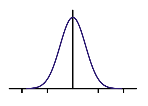
'Gaussian filter'. A one dimensional Gaussian looks like the
function below.
Since we have a 2D image, we use a 2D Gaussian that looks like the
image below.

To smooth the image, we look at a particular pixel. We place a
2D Gaussian centered at that pixel. We then calculate a sum by
multiplying the Gaussian times the image pixel value for each pixel
in the Gaussian. We replace the value of the particular pixel
with the value of the sum. In principle, the Gaussian has
infinite extent in each dimension, but in practice, we limit the
Gaussian and the sum to cover only a finite number of pixels.
The Gaussian is normalized so that its sum over selected set of
pixels is unity. This process is called convolution. The
wikipedia page on convolution, http://en.wikipedia.org/wiki/Convolution,
has a good explanation with some nice graphics to help you get some
intuition about what convolution means and does to functions.
One can do convolution with functions other than Gaussians.
The function selected for convolution with the image is called the
'kernel'. We use gaussian_filter from the
scipy.ndimage.filters package that handles all of these details for
us. That function takes two parameters. One is the image
to be smoothed and the other is the standard deviation for the
Gaussian, which is called sigma. Sigma can be given a single
number, which makes a symmetric function, or as a sequence with a
different value for each axis.
Smoothing will change the range of pixel values in the image.
Thus, after smoothing, we need to re-evaluate the range of
interesting pixel values to use for our plots. Execute the
cell that does smoothing and then plots the smoothed image.
Try adjusting the value of sigma to see what it does to the
plots. Each time you adjust sigma, you may need to adjust the
how vmax is set in order to get a good image. Try values of
sigma of 1, 2, 5, 10, 20, and 50. How would you describe the
effect of different values for sigma on the image? After you
are done, set sigma back to 10.
Contour and surface plots
Contour and surface plots are different ways of presenting
data. They have advantages and disadvantages relative to
images. The choice of which type of plot to use is often
aesthetic and the plots of different types are sometimes
combined. For example, to compare gamma-ray and radio images
of a nebula, one might overlay contours generated from the radio
data on to an image of the gamma-ray data.
To make contour and surface plots in Python, we need three
variables: one that holds the X coordinate of each bit of data (in
our case, the pixel location), one that holds the Y coordinate, and
one that holds the Z coordinate (in our case, the intensity in the
pixel). We have the Z data already in the image. The
first thing that the next block does is generate arrays with the
needed X and Y coordinates. We first generate arrays of
numbers for X and Y. These arrays must have the same length as
the corresponding axis of the image. Our code uses the pixel
number for the coordinate value. You might want to use
something like the astronomical coordinate values instead. We
then take those arrays and combine them into a grid. The
resulting arrays x and y have exactly the same shape as the
image. Each entry gives the x or y coordinate of the
corresponding pixel in the image.
For contour plots, we need to set the contour levels. These
are the pixel values at which the contours are drawn. For
example, if we pick a level of 0.5, the plot will have a contour
that separates pixels with values above 0.5 from those with values
below 0.5. We have chosen to generate contour levels from vmin
to vmax using np.linspace and then drop the values at vmin and vmax
(those contours would be empty, think about it). The selected
levels go into the variables contours. The plt.contour
function makes the contour plot and returns information about the
contours that can then be used by plt.clabel to label the contours.
Surface plots are representations of 3D images. (I am still
waiting for my holographic 3D display.) We need to import
Axes3D from mpl_toolkits.mplot3d to get functions to set up 3D
plots. The plot_surface function then plots surfaces in the
graphical space set up with Axes3D. Note that you can click
and drag in the surface plot window if you want to see the plot from
different angles. It's cool.
Your turn
We used some simple statistics to attempt to adjust the scaling
for our images. Another possible way to scale the data would
be to adjust the lower and upper bound on the scale so that some
percentage of the pixel values lie below the lower bound and some
percentage lie below the upper bound. Modify the code in
plot_image.py so that it takes two parameters, vmin_frac and
vmax_frac, that adjust vmin and vmax so that vmin_frac of the
pixels have values below vmin and vmax_frac have values below
vmax. To start, you might use vmin_frac = 0.01 and vmax_frac
= 0.95, but note that they must be adjustable. Save this
code for your future use.
FYI
The image that we used was downloaded from the Hubble Legacy
Archive (HLA). The HLA is "designed to optimize science from
the Hubble Space Telescope by providing online, enhanced Hubble
products". If you want to plot more Hubble images, you can
access the HLA at https://hla.stsci.edu/hlaview.html.
Type an object name in the box (M16 is a nice one), click on
Search, then click on the Images tab. You can then download
by right clicking (or whatever mac people do) on one of the
FITS-Science links. You should be able to read the FITS file
directly into today's program. However, you'll need to do
some work on setting vmin and vmax as the raw HST images usually
include major outliers.