Lecture #23

Scientific Computing Using Python - PHYS:4905

Lecture Notes #23 - Prof. Kaaret

Homework #17 is at the bottom of this page.

Differential equations

Differential equations occur very often in physics. 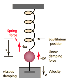Damped oscillator

For example, the motion of the damped, harmonic oscillator shown in the figure to the right is described by the equation

m \frac{d^{x}}{d t^{2}} + c \frac{d x}{d t} + k x = 0

m \frac{d^x}{dt^2} + c \frac{dx}{dt} + kx = 0

where x is the displacement, m is the mass, c is the damping force coefficient, and k is the spring constant.

A differential equation of any order can be converted to a set of first-order differential equations. For the example above, we can introduce the velocity as a new variable,

v = \frac{dx}{dt}

and rewrite the second-order differential equation as two coupled, first-order differential equations,

\frac{dx}{dt} = v \, , \;\;\;\; \frac{dv}{dt} = - \frac{cv + kx

This is the general form that we will use since it is the form needed by the differential equation solvers built into the SciPy library (and also many Fortran and C libraries). We consider a set of first-order differential equations over a set of variables

\{ t, y_i\}

with i = 1, 2, ... N, where the derivatives are set by a set of functions

f_i(t, y_1, y_2, …, y_N)

so that

\frac{dy_i(t)}{dt} = f_i(t, y_1, …, y_N)

Boundary waters

In addition to the differential equation, we need to know the boundary conditions to calculate the behavior of our physical system. There are two categories of ways to set the boundary conditions. The first defines initial value problems. In an initial value problem, one sets the initial values. In the damped harmonic oscillator problem, we would set the initial value of the displacement and the velocity at some time usually taken as t = 0. That would specify the right hand side of our set of equations at that time. We would then use the differential equations to calculate the values of x and v at all later times of interest.

The other way to set boundary conditions is to specify the starting and ending point. These are called boundary value problems. For example, you might specify that the mass should be at zero displacement at t = 0 and then again at t = T. You would then have to figure out the appropriate velocity at t = 0 to make that work out. A more realistic example is that you might want to have your ballistic projectile hit a specific target after being launched from a fixed location. Again, you set the beginning and starting points, but need to find the appropriate initial value for the velocity. Problems involving the calculation of electric fields typically start with specification of a configuration of charges then one needs to find the intervening field. These are also boundary value problems.

For today, we'll concentrate only on initial value problems. They are easier. Boundary value problems require different techniques for their solution.

Euler method

Let's consider the differential equation

\frac{dy}{dt} = f(t, y(t))

with the initial value

y(t_0) = y_0

We can approximate the derivative with a finite difference

y'(t) \, ≈ \, \frac{y(t+h)-y(t)}{h}

We can solve this for y(t+h),

y(t+h) ≈ y(t) + hy'(t)

Using our equation for the derivative,

y(t+h) ≈ y(t) + hf(t, y(t))

To program this, we use h as the step size and construct a time sequence

t_n = t_0 + nh, \;\;\; n = 0, 1, ...

and find the value of y at each time step,

y(t_n+h) = y_n + h f(t_n, y_n) \;\; ⇒ \;\; y_{n+1} = y_n + h f(t_n, y_n) \;\;\;\;\;\;\;\;\; (1)

This is the Euler method. Unfortunately, the Euler method is not very accurate.

You can see why, from the graph to the right (from the Wikipedia page on the Euler method) in which the blue curve shows the correct solution of the differential equation and the red segments show the approximate solution from the Euler method. In the Euler method, the slope of the function is estimated from the start of the interval. One assumes a constant slope over the interval to calculate the next point. If the slope is changing, as in this example, this leads to inaccuracy. Since we don't usually don't actually know the correct solution of the different equation (or we wouldn't be calculating it numerically), the error builds up over time. The local error, or the error per step, is proportional to the square of the step size. The global error, or the total accumulated error, is proportional to the step size. The scaling of error with step size leads to the Euler method being called a first-order method.

Runge-Kutta methods

The accuracy of our estimate for the value of y at the next time step could be improved if we divided up the time step and used multiple function evaluations to improve our estimate of the derivative. In the midpoint method, we divide the step into two pieces. First, we find the value at the midpoint of the interval,

y(t_n + h/2) = y_n + h f(t_n, y_n)/2

Then we substitute that (t, y) position into our integration step equation (1) to get a new equation,

y_{n+1} = y_n + h f\left(t_n + h/2, \; y_n + hf(t_n, y_n) \right)

The global error of the midpoint method is proportional to the square of the step size, so it is a second order method.

This is a significant improvement over the Euler method, but we can keep going to higher orders. Methods of this type are call Runge-Kutta methods. The most widely used Runge-Kutta method is the fourth-order method. It uses a weighted average of four estimates of the slope of the function

k_1 = h \, f(t_n, y_n)

k_2 = h \, f(t_n+h/2, y_n+k_1/2)

k_3 = h \, f(t_n+h/2, y_n+k_2/2)

k_4 = h \, f(t_n+h, y_n+k_3)

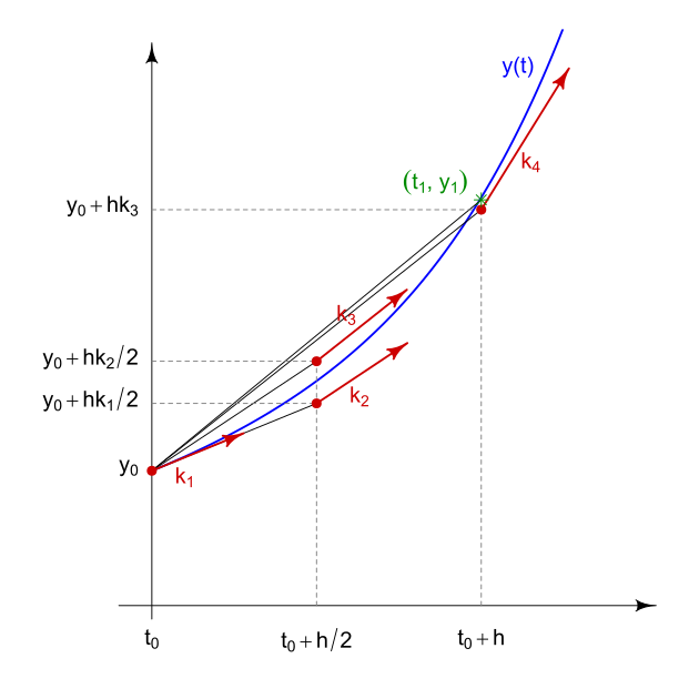
These are shown graphically in the figure to the right (from Wikipedia's page on Runge-Kutta methods). There is a slope estimate from the beginning of the interval, one from the end of the interval, and two from the middle of the interval. Note that the calculation of each slope makes use of the previously calculated slope.

For the integration step, we use a weighted average of these four slope estimates with the ones from the middle of the interval weighted higher.

y_{n+1} = y_n + (k_1 + 2 k_2 + 2 k_3 + k_4)/6

This Runge-Kutta method is fourth order, meaning that the total accumulated error scales as

h^4

. The method is called RK4, the "classical Runge-Kutta method", and "the Runge-Kutta method". RK4 requires four evaluations of the function f per time step to achieve fourth order. The fifth-order Runge-Kutta method requires six function evaluations per time step, and so generally produces a declining return on accuracy achieved versus computation required.

You may recognize the set of coefficients in RK4; they are the same as those in Simpson's rule used for numerical integration. Indeed, if f does not depend on y, then solution of the differential equation becomes a simple integration and RK4 is equivalent to Simpson's rule.

Adapt to the times

To perform accurate numerical integration while minimizing the computation required, numerical quadrature algorithms adapt the grid spacing. The same is true for the solution of differential equations. Adaptive differential equation solvers adjust the step size to achieve the desired accuracy.

To do this, we need an estimate of the accuracy of the integration. This is usually done by comparing two different methods, with one of order p and one of order p-1. For Runge-Kutta methods, this is computational efficient because the two methods have common intermediate steps. If the estimated error exceeds a user-defined threshold, then the step size is decreased and the step is repeated. Conversely, if the error is well below the threshold, then the step size is increased in order to save on computations.

We will be using a Python routine that, by default, uses the "RK45" method for adaptive solution. RK45 does calculations using a fifth-order Runge-Kutta method and checks their accuracy by comparing with a fourth-order Runge-Kutta method. This method works well and is reasonably computationally efficient in most cases. If you have equations that particularly troublesome, then you'll need to read about other methods.

Homework #17

For HW #17, you will write Python code to numerically solve the equations of motion for the coupled oscillators from lecture #22. We have two masses, each with mass m, attached by springs with spring constants as shown in the figure below with x₁ being the displacement of the first mass from its equilibrium position and x₂ being the displacement of the second mass from its equilibrium position.

The equations of motion are

m \ddot{x}_1 = -(k+κ) x_1 + κ x_2

m \ddot{x}_2 = κ x_1 -(k+κ) x_2

We can convert these to a system of first-order differential equations by introducing the velocities,

v_1 = \dot{x}_1, \;\;\; v_2 = \dot{x}_2

Then, we have the system of equations

\frac{dx_1}{dt} = v_1 \, , \;\;\; \frac{dv_1}{dt} = -\frac{k+κ}{m} x_1 + \frac{κ}{m} x_2

\frac{dx_2}{dt} = v_2 \, , \;\;\; \frac{dv_2}{dt} = \frac{κ}{m} x_1 -\frac{k+κ}{m} x_2

We will be using the solve_ivp routine in the scipy.integrate package. This routine calculates the solution of a system of ordinary first-order differential equations given a set of initial values. The problem is defined as

\frac{dy}{dt} = f(t,y), \;\;\;\; y(t0) = y0

where t is a scalar variable, y is an n-dimensional vector, and f is a function that returns an n-dimensional vector giving the derivatives of y at the time t. We will translate our variables into a numpy array by setting the elements of y to be

[x_1, v_1, x_2, v_2]

. Our function is then

def dfun(t, y) : # find derivatives at current time # t = time, not used explicitly # y = vector [x1, v1, x2, v2] # constants defining the system k = 2.0 # [N/m] spring constant for edge springs kappa = 2.0 # [N/m] spring constant for center spring m = 1.0 # [kg] mass of masses # unpack y into physical variables x1 = y[0] # displacement of mass 1 v1 = y[1] # velocity of mass 1 x2 = y[2] # displacement of mass 2 v2 = y[3] # velocity of mass 2 # calculate derivatives dx1dt = v1 dv1dt = -x1*(k+kappa)/m + x2*kappa/m dx2dt = v2 dv2dt =x1*kappa/m - x2*(k+kappa)/m # return derivatives packed into an array return np.array([dx1dt, dv1dt,dx2dt, dv2dt])

Let's start our masses at rest, with the first mass displaced by 0.1 meters in the positive direction and the second by 0.2 meters. Our initial values are then

y0 = [0.1, 0.0, 0.2, 0.0]

Now, let's integrate the equations of motion for 20 seconds. We specify that by using a tuple with the initial and final times

t_span = (0.0, 20.0)

We can now call solve_ivp to do the calculations. The calling sequence is

from scipy.integrate import solve_ivpsol = solve_ivp(dfun, t_span, y0, rtol=1E-6, atol=1E-9)
The variables rtol and atol specify the relative and absolute tolerances on the accuracy of the computation. The solver keeps the local error estimate at each step less than

atol
      + rtol * abs(y)

. You may want to play with these to get better solutions. Also, it is possible to pass arrays if you need to set the tolerances on each component of y individually.

The routine returns a "bunch object" with a bunch of fields. Some of the most useful ones are
sol.t = the time points used
sol.y = the values of the variables at each time point.
sol.success = True if a solution was obtained.

The solve_ivp routine has many optional parameters and many fields that it returns that are described at its reference page https://docs.scipy.org/doc/scipy/reference/generated/scipy.integrate.solve_ivp.html#scipy.integrate.solve_ivp. Of particular interest is the events parameter that you can use to terminate the integration under certain conditions, e.g. if you are integrating the trajectory of a projectile, you can stop the integration when it falls back to Earth. There are explanations and examples for the different options on the reference page.

Using the code fragments above, write a Python program that integrates the equations of motion for a pair of coupled oscillators. Set the masses and spring constants to the values defined in the function dfun. Have your code:

1) Make a plot that could be used to graphically estimate the eigenfrequency for the eigenmode where the two oscillators move in unison and print out your estimate using your plot. Note that you don't have to program in a way to estimate the eigenfrequency. You can do this by hand and then code your procedure and result into the print statement, e.g. "I measured the intervals containing three successive peaks to be 62 seconds, therefore the period is 31 seconds".

2) Make a plot that could be used to graphically estimate the eigenfrequency for the eigenmode where the two oscillators move in opposition and print out your estimate using your plot.

3) Print out the displacement and velocity of each mass at t = 20 s for the initial conditions where the first mass starts displaced by 0.3 meters, the second mass starts at x₂ = 0, and both masses start at rest.

Please hand in your code electronically. This assignment is worth 40 points.