The Earth as a Planet, 2

>>> Inspiring picture of Earth from space.

http://www.solarviews.com/r/earth/earthx.gif

Look at Figure 7.6 to see where the plates are.

>>>>>> Map with tectonic plates.

Let’s look again at the motion of these plates over geological time.

http://www.ucmp.berkeley.edu/geology/anim1.html

The fundamental reason for this plate motion is convection of the mantle material. The tectonic plates float on these convection cells. >>>> transparency with convection, continental drift.

Types of Plate Motions

Remember, in an astronomy class we are talking about all of this to grasp it as a potentially general, widespread planetary process! Transparency with these processes.

· Rift

· Subduction

· Mountain building and plate collision

· Faulting and plate shear

Question for the august assembly: What are some of the well-known phenomena associated with these motions?

One of the most fascinating aspects of continental drift is the consequences for the geography of the Earth during the Permian Period. Our models of continental drift indicate that the location of the continents relative to each other has changed during the geological history of the Earth. Two hundred and fifty million years ago (the Permian period) all of the continents were shoved together in a supercontinent termed Panagea. The rest of the Earth was covered by a superocean termed the Panthalassic Sea.

http://www.scotese.com/pg280anim.htm

Radioisotopes and Ages of Rocks (Rocks of Ages?)

Today I will start talking about one of the most important concepts in solar system astronomy. How do we determine how long ago solar system objects came into existence? More generally, how do we put “time stamps” on events in the remote past?

This material is on p138, Chapter 6 of your textbook, but I will be putting a lot more info than is there.

The technique used is radioisotope dating, and the basic idea is used in archaeology as well as planetary science. Here goes.

Elements are determined by the number of protons in the nucleus, i.e. 6 for carbon, 7 for nitrogen, and 37 for Rubidium. It is this atomic number that determines its chemical characteristics.
In nature, elements have a number of isotopes, in which the atomic nuclei have the same number of protons, but different numbers of neutrons. Neutrons are subatomic particles which have the almost the same mass as a proton, but no electric charge. So the atomic weight of the isotopes differs.
Examples: Seawater on Earth consists of H₂O. The vast majority of the hydrogen atoms are plain old hydrogen, ¹H, but about 150 out of a million atoms is Deuterium, ²H or D, in which the nucleus has a proton and a neutron. Another famous example is carbon, in which the most common isotope is C¹², but C¹⁴ is present as well.

Some isotopes are stable, meaning that once formed, they will last forever. However, some of them are radioactive, meaning that they transform themselves to a different type of nucleus, and emit nuclear radiation in the process.

An example of a radioactive decay process is

₃₇Rb⁸⁷→ ₃₈Sr⁸⁷ + β + ν

For a given Rubidium atom, the decay process shown here is random. It could occur tomorrow or a billion years from now. However, statistically, a group of these atoms will decay at a rate such that after one half life, half of them have decayed and half remain.

After another half life, half of the ones left before will decay. After another half life, half of half of half will be left, and so on.

This statistical behavior is a consequence of the fact that atomic nuclei are governed by quantum mechanics, a branch of physics that has a distinctly probabilistic nature.

The crucial fact to emphasize is that every group of radioactive nuclei in the universe will have the same radioactive decay characteristics, with the same half life.

Say it with equations!

The equation describing radioactive decay is:

N(t) = N₀e^-0.693t/T

► Show transparency with exponential decay.

How Can We Use Radioisotopes as Clocks

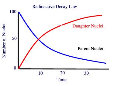
A rock will form with atoms of various elements and isotopes. Once the rock forms, they are stuck there. The atoms which form the rock will include some radioisotopes. Once the rock has formed, the radioisotopes will begin to decay from the parent nucleus to the daughter nucleus. By comparing the number of daughter nuclei to parent nuclei, we can determine the time since the rock formed.

Example: Parent isotope A decays to daughter isotope B in 10 million years. When the rock forms, it has 100 atoms per cubic centimeter of isotope A, and none of isotope B. After 10 million years, there are 50 per cc left of A. The rest have changed to B, so we have 50 of each. After another 10 million years (another half life, 20 millions years after the rock has formed, only 25 of the 50 A atoms are left; the other 25 have gone on to an afterlife as B atoms, so we have A: 25 B: 75. After another half life (30 million years after the rock formation) we have 12 of A and 88 of B. Thus by counting the relative numbers of A and B we can tell how long it has been since the rock formed.

>>>>>>>> Sketch on Blackboard of A(t) and B(t) curve.

To use radioactivity for dating (or age determination) you need a radioisotope with a half life in the ballpark of the age of the objects you are interested in. For example, Carbon 14 dating uses the reaction

C¹⁴ → N¹⁴ + β + ν

This reaction has a half life of 5600 years, and is therefore useful for archaeological dating.

For geological and astronomical applications, we need radioactive decay schemes with much longer half lives. Some of the reactions used in astronomy are given in Table 6.3 on p139 of your book. Note the Rubidium-Strontium reaction with a half life of 48.8 billion years, and the Potassium-Argon, with a half life of 1.31 billion years.

By the size of these numbers, you can conclude that the ages of rocks (on the Earth and elsewhere) are quite large.

Concluding Remarks

(1) Der Garten der Zeit in Mainz, Germany.

(2) Question for the august assembly: How can we assume that there is nothing (not a trace) of the daughter isotope when the rock forms? How will an initial presence throw off the basis of dating? How can we correct for the fact (for example, that Strontium 87 would already be present in the rock when it formed) and get a credible estimate for the age of the rock?