Signal versus Noise

Astronomical Laboratory 29:137, Fall 2013
by Philip Kaaret

Reading

Sections 4.3-4.5, 5.1, and 5.4 in Handbook of CCD Astronomy, second edition, by Steve B. Howell.
Santa Barbara Instruments Group ST-402ME CCD camera
SBIG CCDOps manual
Kodak KAF-0402E/ME CCD

Introduction

In this lab, you will calculate the signal to noise ratio of a stellar brightness measurement made with a CCD cameras.

Equipment

An SBIG ST-402XME camera, with power adapter and USB cable
A computer running the CCDOps software package and DS9 for image analysis

Signal and Noise

A ideal imaging detector for astronomy would record the number of photons striking each pixel and nothing else - no counts due to read noise or dark current. As you found in the previous lab, the measurements produced by a CCD will also have contributions due to noise associated with the electronics that amplifies and digitizes the charge signal in the CCD readout (read noise) and due to electrons released by thermal fluctuations in the silicon (dark current). In order to measure the brightness of a star these contributions must be measured and subtracted off. However, since the read noise and dark current arise due to random process, they will fluctuate and it will never be possible to subtract them off exactly.

Steps in CCD Data Reduction

The standard steps in the 'reduction' of an astronomical image are as follows:

Subtract a mean dark frame from the object frame
Divide the resulting frame by a dark subtracted mean flat field frame

One then ends up with a 'reduced' object image that has been corrected for the CCD effects of bias and dark current and for variations in the quantum efficiency across the field of the CCD and telescope.

To do photometry on a star, one then draws a circle around the star and sums up the counts inside the circle. Since the night sky is not perfectly dark, one also draws an annulus centered on the star and excluding any other stars and then subtracts the contribution from the sky background. The radius of the circle enclosing the star should be selected to include most of the counts from the star, but not be so large that it includes too much sky background. The inner radius of the annulus should be large enough that it does not include any counts from the star. The total area of the annulus should be a few times larger than that of the circle.

CCD Signal to Noise Equation

The signal, S, from the star is the total number of net electrons, N_*, recorded by the CCD from the star after subtraction of the bias, dark current, and sky background. The generation of each electron is a random process and if we take repeated measurements of the star the value of N_T will fluctuate according to a Poisson distribution (note that we use N_T instead of N_* as in the textbook). In the limit of large N_T (acutally N_* > 25 is enough), the Poisson distribution is well approximated by a Gaussian distribution and we can describe the fluctuations in N_T in terms of a standard deviation equal to sqrt( N_T). This is true even with an ideal CCD and telescope and with zero sky background. These instrinsic fluctations contribute a limiting noise term σ_* = sqrt( N_*). A 'bright' source is defined as one where the intrinsic noise dominates and, thus, the signal to noise ratio, S/N, for a measurement of the source is

S/N = N_*/sqrt( N_*) = 1/sqrt( N_*)

The number of electrons recorded by the CCD from the dark current and the sky background are also Poisson distributed and fluctuate in the same way. Let's look at each pixel individually, we write the number of dark current electrons per pixel as N_D. Even though we subtract off an estimate of this number, the fluctuations in the number of dark current electrons remains and adds noise per pixel, σ_D = sqrt(N_D). The same is true for electrons produced by the sky background. The number of electrons per pixel from sky background is N_S and each adds noise, σ_S = sqrt(N_S).

The read noise, σ_R, is the noise associated with the electronics that amplifies and digitizes the charge signal in the CCD readout. Read noise is present even for zero signal and is usually assumed to be independent of the magnitude of the signal. Read noise will arise for each pixel in the star image, so one needs to sum up the read noise for all the pixels in the source extraction region.

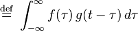
We are then led to the question of how to add these various noise contributions. The key point is that the noise distributions are well described by Gaussian probability distributions. To combine two probability distributions, one performs a convolution. The convolution of f and g is written f∗g. It is defined as the integral of the product of the two functions after one is reversed and shifted:

$http://upload.wikimedia.org/math/1/8/5/185ff6a342b3ec1719643396613151e2.png$ $\stackrel{\mathrm{def}}{=}\ \int_{-\infty}^\infty f(\tau)\, g(t - \tau)\, d\tau$

The wikipedia page on convolution, http://en.wikipedia.org/wiki/Convolution, has a good explanation with some nice graphics to help you get some intuition about what convolution means and does to functions.

The convolution of two Gaussians is another Gaussian. If the width (standard deviation) of the initial Gaussians are σ₁ and σ₂, then their convolution has a width σ² = σ₁² + σ₂². This sort of addition is called "root of sum of squares" or "addition in quadrature". Noting that we need to sum up the noise contributions from dark current, sky background, and read noise for each pixel in the circle containing the star, i.e. for n_pix pixels, the total noise is then:

σ² = σ_T² + n_pix × (σ_S² + σ_D² + σ_R²) = sqrt[N_T + n_pix × (N_S + N_D + σ_R²)]

Contrary to what is stated in the textbook, the reason that the read noise term appears with a square, unlike the other terms in the expression on the right, is simply because it is a directly measured noise, while the other terms are estimates of noise derived from a number of electrons, e.g. σ_S = sqrt(N_S). Note that the noise terms are uniformly treated in the center expression. (Also, note that 'shot noise' is another name for 'Poisson noise', so the footnote on page 74 actually makes no sense.) The signal to noise equation for CCDs or the "CCD equation" is then:

S/N = N_*/sqrt[N_T + n_pix × (N_S + N_D + σ_R²)]

In the previous lab, you measured the read noise of the SBIG ST-402 and how the dark current depends on temperature and exposure time. In this lab, you will use the images that you obtained of Vega to estimate the sky background and the signal level from stars and you will use the dark frames to estimate the dark current. Using this information, you will then plot how the S/N depends on various parameters.

Measuring Counts from Vega, the Sky, and the Dark Current

The goal in this section is to use the images that you obtained while observing Lyra on the roof to measure the counts from a selected star, the sky background, and the dark current. Note that you need a sky image that does not have a dark frame subtracted, a dark frame with the same exposure time and temperature, and a bias frame (dark frame with 0.040 second exposure) at the same temperature.

Load an image of Lyra obtained with the R filter into ds9. Pick the brightest star in your image that is not saturated, i.e. the image contains no pixels with values above 30,000. Do not use Vega if it is saturated (which is it on many team's images). You may want to set the image scale to logarithmic (Scale/Log) and play with Scale/Scale Parameters.
Zoom in on your star so that you can see the individual pixels. Draw a circle around the star that contains most of the counts from the star. In ds9, do Region/Shape/Circle, then left click at the center of the circle and drag out to your desired radius. If you want to adjust your circle after drawing it, left click inside and you can then move and resize. Doubling left clicking inside brings up a dialog box where you can adjust the parameters by hand.
Now draw an annulus centered on the star. Use an inner radius large enough not to include any counts from the star and an outer radius so that the area of the annulus is several times the area of your circle, but avoiding any stars visible.
If you drew a bunch of extra regions, go and delete them now.
Save your regions: Region/Save Regions. Pick a file name of your choice and use ds9 format and physical coordinate system.
Left-click on your circle, then do region Region/Analysis/Get Information/Statistics. This should bring up a new window with information about the region and the counts inside. Record the 'sum', which is the sum of the image counts in the region, and the 'area', which is the number of pixels in the region.
Do the same for the annulus.
Now load a dark frame into ds9 taken with the same exposure time and same CCD temperature as your R-band image (File/Open). If you want to look at both frames simultaneously, do Frame/New Frame before loading the dark frame and then afterwards do Frame/Tile Frames and then Frame/Match/Frame/Physical. You might want to re-size your ds9 window to see both images.
Load the regions from your sky image into the ds9 frame with the dark image - do Region/Load Regions, use ds9 format and 'Load into Current Frame'.
Find and record the statistics (sum and area) for the circle and annulus on the dark frame. Note that the area for the circles should be the same in both images (also for the annuli).
Now do the same for the bias frame. Find and record the statistics (sum and area) for the circle and annulus on the bias frame.
Usually, one does the bias and dark subtraction on a pixel-by-pxiel basis, but here we will do it by hand. First, do the bias subtraction: take the number of counts for the circle and the annulus for the sky and dark frames and subtract off the corresponding number of counts in the bias frame. Record those. Also calculate the number of dark current counts per pixel. Do this by dividing the number of bias-subtracted counts in the annulus in the dark frame by the number of pixels in the annulus.
In the previous lab, you produced plot of dark current versus temperature for the ST-402. Using that curve, estimate the dark current counts per pixel that you should have found in your image given the CCD temperature and exposure time used. Do they agree?
Now we'll do the dark subtraction. Take the numbers that you just found and subtract the (bias-subtracted) counts from the dark frames from the (bias-subtracted) counts from the sky images. Calculate the number of sky background counts per pixel.
Now we need to subtract the sky background. Calculate the sky background per pixel = (dark-subtracted counts in the annulus)/(number of pixels in the annulus). Multiply by the number of pixels in the circle and subtract that number from the dark-subtracted counts for the star. You now have the net number of counts from your star. Record your calculations.

Calculating the Signal to Noise Ratio

Now let's calculate the S/N of your detection of your selected star. You just calculated values for N_T , N_S, and N_D in counts. Recall that you need to convert these to electrons. Use the gain of the CCD (that you can readoff using CCDOps or get from your write-up of the last lab) to do this conversion. In choosing the radius of the circle that you used to extract counts for the star, you picked n_pix . Use your value for the read noise, σ_R², from the previous lab. Record your calculations and your results in your lab notebook. Which component of the noise dominates?

Go back to your sky image and change the radius of the circle to be 1, 2, 3, 4, and 6 physical pixels (if your original radius was not less than 6 pixels, see the instructor before picking the set of radii). In each case, record the sum of counts and number of pixels in the circle for the each image. Writes a short Python program that takes these values in arrays and makes 1) a plot of the net counts for the star versus extraction radius, and 2) a plot of S/N versus extraction radius. Note that you don't need to repeat the measurements for the annulus (as long as its inner radius is large). You don't need to repeat the annulus calculations each time

Now inspect your sky image and find a much dimmer star, one of the dimmest that you can see. Repeat the process above, ending up with a pair of plots (as above) for the dimmer star.

Put printouts of your four plots in your lab notenook and write some discussion comparing them with figure 5.6 and the upper panel of figure 5.7 in the textbook.